Oh boy, this is going to be a doozy of a blog post.
I’ve spent the last three months in New York1 at the Recurse Center, developing an understanding of the fundamentals of digital photography.
Something that’s been really, really rewarding about this project is that I’ve been able to take my own images, start with the actual bits in a hex editor, and interpret them into images that progressively become more faithful and more beautiful, the more code I write.
Well, almost. There was one minor hiccup – all of the RAW files I’ve shot over the last 3 years have been encoded with Fuji’s lossless image compression algorithm. This is a fantastic technology as a photographer – 50 MB files are swiftly reduced to 25 MB, with literally no reduction in quality – but if you’re writing your own processor, then you need to decompress the data, and compression algorithms are usually complex.
When should you implement something yourself?
I knew that this was going to be a rabbit hole before I started. I could hear the voice of my former boss saying “Fabian. Do you really need to be doing this?”.
I’ve written about Yak Shaves before, and in theory I should know better – but, part of what attracted me to the Recurse Center in the first place was it seemed like a place where going down rabbit holes was permitted. Maybe not advised, but definitely permitted. So, in the first week of February, I found myself trying to figure out how Fuji’s lossless image compression technology worked.
The thing was, I already had the ability to load compressed Fuji RAF files in my software – the excellent, albeit minimally documented, LibRaw project has had support for this since 2016, and my code was initially loading files by binding to LibRaw. At some point, though, I got frustrated with not knowing exactly what was in my RAW file. Libraw is functionally very good, but it doesn’t do a good job of surfacing what its sources are for any given piece of data2. One thing led to another, and at some point I’d decided to replace LibRaw with my own code. Which meant I’d need to re-implement Fuji’s lossless compression algorithm, at least for the photos from my specific camera model.
How does it work?
Fuji RAF lossless compression can be characterised as an adaptive, differential compression algorithm. Let’s break that down:
- Adaptive: the algorithm changes with the data it has processed in the past
- Differential: the algorithm is predicated on storing the difference between an ’expected’ value and the actual value.
Step 1: Split into stripes
First, split the image into a set of vertical stripes. My camera (the Fuji X-T2) uses 8. Each of these stripes is encoded independently (i.e. with separate input, output, and state), which means it’s possible to parallelise the encoding and decoding. This turns out to be super important for performance on modern CPUs – parallelising my decoder resulted in a 6x speedup in user time (on a 4-core hyperthreaded machine).
Splitting the image into vertical stripes
Step 2: Sensor data → Colored vector collation
Now that we’ve split the image into stripes, we can break each stripe down further into lines of nx6 pixels. We’ll take each of those lines, and map their pixels into color vectors. It’s probably easiest to explain this with a diagram:
Mapping Sensor Pixels to Colored Blocks
If you’ve never worked with digital imaging before, you might be surprised that each pixel in a camera sensor only represents one color. The pixels themselves aren’t capable of differentiating between different colors of light, just of counting approximate numbers of photons, so manufacturers usually slap a Color Filter Array on top to narrow the color range that each pixel responds to.
We collate the pixels by color because later, we’ll apply a transform that encodes the differences between neighbouring pixels. If the neighbouring pixels all represent the same component color, those differences are smaller, which allows for better compression.
Now that we’ve got the data collated into solid color blocks, we’re ready to start processing.
Step 3: Color vectors → bits
Here’s where it gets real interesting. Now that we’ve collected the data into color vectors, we interleave two color vectors and compress them together.
Let’s use R0 and G0 as our first pair of color-lines. We now need to iterate through each item of R and G, but the order is kinda special:
R[0], G[0], R[2], G[2], R[4], G[4], R[6], G[6], R[1], G[1], R[8], G[8], R[3], G[3], …
We start by iterating through the even slots in R and G. After we’ve done the first 4 of each, we can also start iterating through the odd slots, which will always be 5 positions behind the even slots.
Here it is again in diagram format:
Iteration Order. Notice that we start jumping back to the odd pixels after we’ve started with the even pixels.
This feels weird, but hold with me, we’ll be able to explain it very soon! I promise.
Making a sample for a single value
Now, the idea for a single value is:
- Figure out an expected value for the cell, by (approximately) taking a weighted average of the already processed values around it
- Compute the difference between the actual value and the expected value
- Encode the difference and send to output
- Adapt the encoding process so that it gives better compression ratios in future.
Let’s examine each of those steps individually:
Computing an expected value
Loosely, the expected value of a cell is computed as a weighted average of values around it. What’s vital about this, however, is that these are values that we’ve already processed, because when we’re decoding, we’ll use expected value + difference to compute the output value. The decoder will need to be able to compute the expected value, which means that the encoder can only use values it’s already decoded to compute an expected value.
The details of this are probably better represented in code, but here’s a visual indication of the cells we’re selecting for the weighted average. For even cells, we select these:
Reference pixels for computing Weighted Average, for even-indexed pixels
And for odd cells, it’s these:
Reference pixels for computing Weighted Average, for odd-indexed pixels
This reveals a couple of important ordering dependencies:
- Part of the reason why we don’t start iterating on odd cells until we’ve done a bunch of even cells is because we need the even cells to be processed in order to process the odd cells3.
- To compute the weighed average for each row, we need the values of the previous two rows.
The specifics of the weighted average formulas feel pretty esoteric to me. I’m inclined to suggest that engineers within Fuji were trying stuff out to see what gave the best compression ratios across a bunch of different sample images, found something that worked and was low-cost, and baked that in to the format4.
Compute the difference
This is straightforward! The difference is simply actual_value - expected_value. 🎉
Encode the difference
Because photographic images tend to have big blocks of color, and to change slowly across the image, it’s typically possible to represent the difference from the weighted average in less bits than are required to store the value directly. For an image where every pixel is encoded with 14 bits, we can typically represent the difference between neighbouring pixels with maybe 5 or 6 bits.
Unfortunately, we can’t simply store the differences and call it ‘done’ – just because the differences are typically low, it doesn’t mean they’re always low, and in order to capture every possible difference from the weighted average, we require the same number of bits as we had to start with. We’re going to need a clever encoding scheme to handle this discrepancy.
Let’s say that we’ve got a difference of 27 from the expected value. We’ll represent that in binary as:
11011
Now, let’s say that most of the time, it only requires 6 bits to encode the difference between neighbouring pixels. We’d pad the binary number out to 6 bits:
011011
… but we still need to encode whether we should add or subtract from the expected value. So let’s use two’s complement. We now need to encode 2x the range of numbers (positive and negative), so we need to add another bit. For our example of adding to the expected value, this just means we need to add another zero at the front:
0011011
If we needed to instead subtract 27, we’d use:
1100101
With this 7-bit scheme, we could encode differences between -128 and +127 from the expected value.
Variable Length Codes
So, what should we do if we need to encode a difference outside of this range?
Let’s say that we need to encode a difference of 300 in our 7-bit scheme. We’ll start by converting to binary, which requires 10 bits as a signed two’s complement integer:
+300 = 0100101100
Now, let’s split on the 7-bit boundary. We know we can store the last 7 bits using the scheme we already have:
???
|   7-bit fixed width
|   |
010 0101100
So we’ve got 0b010 remaining at the front. That translates to 2 in decimal, which is a pretty small number. It’s worth noting that we’d expect it to be less likely for this overflow to be a 3, and even less likely again for it to be a 4, or 5, or a 6, because in general, we’re expecting the differences to be small.
This sounds like the perfect candidate for a variable length code. In fact, this is exactly what the algorithm does, converting the ‘2’ prefix into two 0s, followed by a 1:
     2 zeros
     |  terminating one
     |  |
2 => 00 1
Similarly:
5 => 000001
4 => 00001
3 => 0001
2 => 001
1 => 01
0 => 1
Simple, right? And now, we can encode our difference of 300 as:
        [variable-length]
        |
        |   [7-bit fixed-length]
        |   |
+300 => 001 0101100
For a difference of +300, we’re still only paying 3 + 7 bits = 10 bits, instead of the usual 14 to encode a full sample.
When two’s complement isn’t the right tool for the job
We’ve made a problem for ourselves now: notice how we effectively ‘dropped’ the leading sign bit when we converted to variable length?
Consider the encoding of the following two numbers using our scheme thus far:
        [two's complement]      [encoded]
+300 => 0100101100 (10 bits) => 001 0101100
-212 =>  100101100 ( 9 bits) => 001 0101100
Oh, they’re identical! That’s bad! We’re not sufficiently able to distinguish between smaller negative numbers and larger positive ones. It turns out that two’s complement encoding implicitly relies upon the size of the memory in which it is encoded, and our variable coding system drops that information, because it only encodes a single number.
So, let’s throw away our earlier choice of using two’s complement, and use a signed magnitude representation, storing the sign bit at the end, as part of the ‘fixed-length code’ section5. Let’s try encoding +300 and -212 again.
+300 => 100101100     [unsigned binary, 9 bits]
     => 1001011000    [add sign bit to end]
     => 100 1011000   [split on 7-bit boundary]
     => 00001 1011000 [encode using variable length code]

-212 => 11010100      [unsigned binary, 8 bits]
     => 110101001     [add sign bit to end]
     => 11 0101001    [split on 7-bit boundary]
     => 0001 0101001  [encode using variable length code]
Much better! They have different representations now.
Failsafes for large differences
You might have noticed that we’re getting pretty close to our original 14-bit sample size by this point. Indeed, for 14-bit samples, the worst-case difference will be that we’re off by 2^13 - 1 = 81926, and if we try to represent that using our variable length coding scheme, we’ll get:
+8191 => 1111111111111   [unsigned binary, 9 bits]
      => 11111111111110  [add sign bit to end]
      => 1111111 1111110 [split on 7 bit boundary]
      => 00000000 00000000 00000000 00000000
      .. 00000000 00000000 00000000 00000000
      .. 00000000 00000000 00000000 00000000
      .. 00000000 00000000 00000000 00000001
      .. 1111110 🤔      [encode using variable length code]
At some point much earlier, it probably would have just made sense to somehow write that we wanted to directly encode the 14-bit difference instead of using the variable length system for this number.
Fuji’s encoding scheme has a failsafe mechanism for this – if you end up writing 41 or more consecutive zeros, then stop appending zeros and encode the 14-bit delta directly. But… 41 still seems like an awful lot, right?
The problem is, you need a way of encoding the failsafe into your scheme, too. You could, for example, add a ’type’ bit to every value to indicate whether it was absolute or relative. Then, your format would become something like:
         use variable code
         |
         | variable length part
         | |
         | |    fixed size part
         | |    |
 -212 => 1 0001 0101001
+8191 => 0 01111111111111
         | |
         | 14-bit two's complement difference
         |
         use 14-bit direct-encoded difference
But then you have a new problem: you’re effectively paying a whole extra bit on every sample for something you need extremely rarely. A single bit doesn’t seem like a lot, but on a 24 Megapixel image, it adds up to 3 MB per photo (!!).
In general, this is the line of thinking that compression schemes follow. It’s a tradeoff between “how much is this going to cost” vs “how often am I going to need to pay this cost?” I guess ‘41 bits’ is the tradeoff that Fuji picked, probably experimentally, to get the best performance out of the image7.
Now that we’re talking about cost vs frequency, it’s probably a great time to talk about choosing a threshold for splitting between the Variable-Length and Direct-Binary coding schemes.
How Big Should your Direct Binary Coding Section be?
Earlier, we stated:
let’s say that most of the time, it only requires 6 bits to encode the difference between neighbouring pixels.
That assumption’s served us well, but it’s time to admit that it’s not correct enough of the time. The optimal number of bits changes from image to image. Consider – for an image that’s entirely a single colour, you could encode the difference between each pixel as 0, which requires exactly 0 bits to store, whereas for an image where pixel values alternate between 0 and 8191, every delta will be 14 bits (13 bits for 8191, +1 including the sign).
Further, assuming a fixed number of bits works best when photos are consistently variable across the whole frame, and they’re usually not. How many photos have huge swathes of blue sky in them and then details in the foreground?
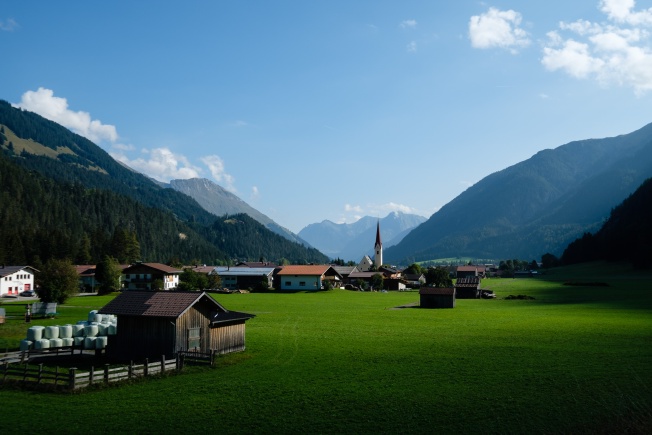
Somewhere near Bach, Austria, September 2018
And like, what about photos with lots of background noise, because they were shot at night at ISO 12500?

I guess there was a full moon that night.
Let’s make it ADAPTIVE
Rather than choose a constant number of bits for the “direct-encoded” part of each value, we can set things up so that the number of bits changes in response to the input. Then:
- Areas with higher local contrast get more bits to encode differences
- Areas that are all the same color can be more efficiently compressed.
I know very little about these schemes in general, but I do know what I read in the LibRaw source code. Here’s approximately how it works:
- Figure out “how much the image is changing in a horizontal direction” by subtracting two known horizontal neighbours
- Figure out “how much the image is changing in a vertical direction” by subtracting two known vertical neighbours
- Quantize those two values into one of 81 “buckets”, which represents the approximate direction and magnitude of change in the image.
Let’s illustrate the steps so far with an example:
Choosing a bucket from neighbouring pixel. The bucket at position (-3, +2) is chosen.
Now, each bucket has been sneakily summing up all the Differences From Expected Value as we’ve worked our way across the image, and counting the number of values that have fallen into that bucket. From these two values, we can:
- Compute the Average Difference corresponding to that bucket,
- Use the number of bits that it would take to encode the Average Difference for the “direct binary coded” part of the output format, and
- Update the Average Difference with the Difference we just encoded.
The end result of this is that the algorithm is able to “learn” how many bits it will probably need to encode the difference for various patterns in the photo. All going well, this should mean that very few bits are required to encode areas without a lot of variation, and areas with a lot of variation are encoded maximally efficiently, i.e. using as much direct encoding, and as little of the expensive variable encoding, as possible. ✨
Step 4: Ship the bits, and we’re done!
Now that we’ve encoded the value, we send it to output. Save it in a file, or send it across the network, it doesn’t matter! It’s not our problem anymore 🎉
Congratulations, you now know the fundamentals behind a very specific photographic compression algorithm.
How effective is this algorithm?
Yeah, that’s a great question! I really don’t know how to quantify that, but I can say that it consistently offers smaller files than the default compression in the Digital Negative format (which is why I’m still using compressed RAF).
On average, my Fuji X-T2 camera will produce a 50.5 MB uncompressed RAF file, of which 49.7 MB is actual RAW data. The values in this file are 14-bit, padded to 16-bit, so if we simply packed all the bits in, we’d be down to about 43.5 MB. Of the photos I’ve shot over the last few years, they typically contain between 21 and 27 MB of compressed RAW data, so I guess we’re seeing a ~35-50% reduction. Not bad, I guess!
It’s worth noting briefly that there are lots of other considerations when evaluating a compression algorithm, like compress / inflate performance and ease of implementation. But if I’m going to talk about that, I’d rather save it for a future blog post.
What about Decompression?
To decompress the image, follow the same steps but in reverse 😉
Ok, not quite. I initially set out to only write decompression code, but I personally found it valuable to implement compression first, in order to better understand why some of the code I was writing needed to be there. Compression and Decompression are two sides of the same puzzle, I guess.
The critical point at which I finally felt like I understood what was going on in this algorithm was when I’d figured out that the Adaptive Coding / Average Difference / Bucketing Subsystem operates in the same direction for both compression and decompression. Think of it like a checksum or a hash: you only ever calculate them in one direction, regardless of whether you’re reading or writing the data.
Was all of this a good use of time?
This project took me around 4 weeks, all told:
- About a week to figure out what the hell was going on
- About two weeks writing my own implementation
- About a week writing this blog post8.
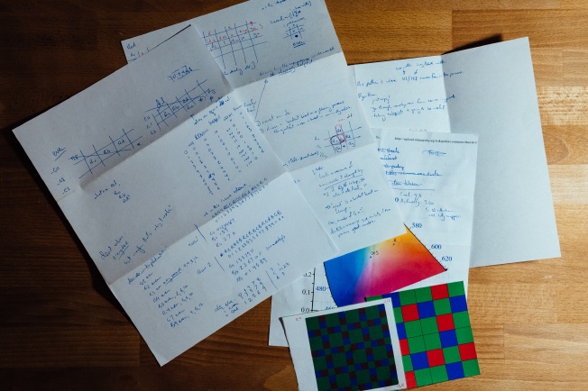
“About a week to figure out what the hell was going on”. These are just the notes I kept 😐
I think it was worth it.
There’s a couple of reasons why I’m still excited about this work:
- Some team of engineers at Fuji spent months designing a compression algorithm, thinking through lots of fiddly, complex pieces along the way. There’s something really nice about taking the care and time to observe all the little decisions that were made, and to wonder about what circumstances led to the specifics. I’ve also learned so many cool little tricks from this project.
- At the flea market in Berlin, you can buy other people’s old reels of film negative. It’s kinda weird and creepy, but I really like the idea of history being available if you look hard enough for it, and it’d be a real shame for every digital photo compressed with this algorithm to turn to noise one day. If you’re a future Digital Archeologist reading through this page, hi! I hope you found this helpful9.
Resources
Hopefully you learned something from this piece! If you’re after more detail, then please accept my sympathies, and these links:
- The libraw source, which has a C++ implementation of the decompression algorithm, and is how I figured all of this out.
- My own Rust implementation in the capnfabs/blitz repo.
If you have questions or feedback, or want to know when I publish more stuff about how digital photography works, feel free to get in touch.
It is, however, open source! So you can figure it out by reading the code. ↩︎
I’m still not sure why we require 3 even cells to be processed before we process the first odd cell, but I’d wager it’s got something to do with parallelisation. The cameras implement encoding and decoding in silicon, so maybe when decoding it takes a couple of cycles for the “East” value to become “available”. ↩︎
Notably, “not a lot of cost” in silicon is very different to “not a lot of cost” in x64 instructions, and the conditionals in this statement probably run pretty quickly on parallel hardware, but they wreck branch prediction when encoding / decoding on a modern CPU. ↩︎
Remember, we allocated a sign bit in the previous section anyway! So we don’t need to add an extra bit for this. ↩︎
Assuming we’re allowed to use wrapping addition / subtraction, and have built something into our encoding scheme to replace -0 with -8193. ↩︎
There might be other factors leading to this choice, too! A maximum of 41 allows everything to fit inside a 56-bit / 7-byte buffer, for example, and maybe that’s a limitation in the compression system on the camera. ↩︎
I had the first version done in two days, but then kept discovering that I didn’t quite understand the reason for something, and having to go back and explore some more. Also, those animations were painstaking. ↩︎
And that you’ve got a way of rendering animated SVGs 😅 ↩︎